POLYNOMIALS AND SPLINES

1. Fitting a polynomial regression

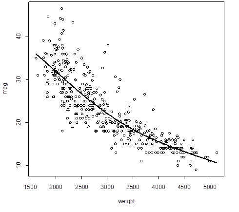
> attach(Auto);

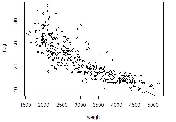
> plot( weight, mpg )

> reg = lm( mpg ~ weight )

> abline(reg)

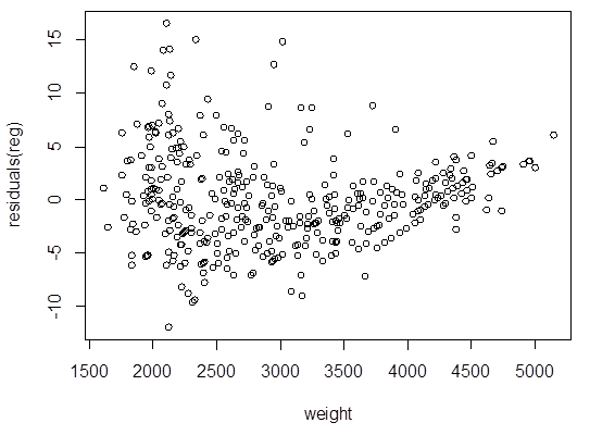
# Look at the residuals. Is linear model adequate?

> plot( weight, residuals(reg) )

# If a polynomial regression is appropriate, what is the best degree?

> install.packages("leaps")

> library(leaps)

> polynomial.fit = regsubsets( mpg ~ poly(weight,10), data=Auto )

> summary(polynomial.fit)

poly(weight, 10)1 poly(weight, 10)2 poly(weight, 10)3 poly(weight, 10)4 poly(weight, 10)5 poly(weight, 10)6

1 ( 1 ) "*" " " " " " " " " " "

2 ( 1 ) "*" "*" " " " " " " " "

3 ( 1 ) "*" "*" " " " " " " " "

4 ( 1 ) "*" "*" " " " " " " " "

5 ( 1 ) "*" "*" " " " " "*" " "

6 ( 1 ) "*" "*" " " " " "*" "*"

7 ( 1 ) "*" "*" " " " " "*" "*"

8 ( 1 ) "*" "*" " " "*" "*" "*"

poly(weight, 10)7 poly(weight, 10)8 poly(weight, 10)9 poly(weight, 10)10

1 ( 1 ) " " " " " " " "

2 ( 1 ) " " " " " " " "

3 ( 1 ) " " " " " " "*"

4 ( 1 ) "*" " " " " "*"

5 ( 1 ) "*" " " " " "*"

6 ( 1 ) "*" " " " " "*"

7 ( 1 ) "*" " " "*" "*"

8 ( 1 ) "*" " " "*" "*"

> which.max(summary(polynomial.fit)$adjr2)

[1] 4

> which.min(summary(polynomial.fit)$cp)

[1] 3

> which.min(summary(polynomial.fit)$bic)

[1] 2

# BIC chooses a quadratic model “mpg = β₀ + β₁ (weight) + β₂(weight)² + ε”. Mallows C_p and adjusted R² add higher order terms.

# Cross-validation agrees with the quadratic model…

> library(boot)

> cv.error = rep(0,10)

> for (p in 1:10){

+ polynomial = glm( mpg ~ poly(weight,p) )

+ cv.error[p] = cv.glm( Auto, polynomial )$delta[1] }

> cv.error

[1] 18.85161 17.52474 17.57811 17.62324 17.62822 17.69418 17.66695 17.76456 18.35543 18.59401

> plot(cv.error); lines(cv.error)

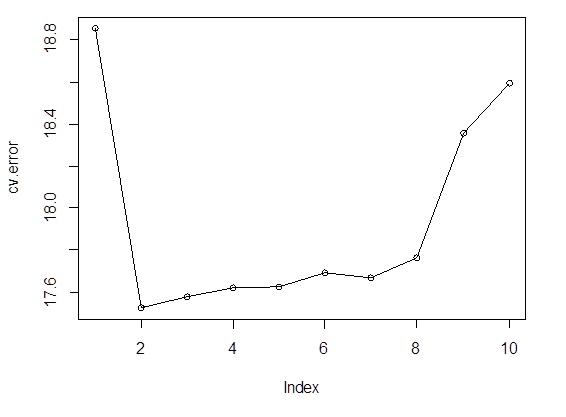
# So, we choose the quadratic regression – degree 2 polynomial. Its prediction MSE is 17.52.

> poly2 = lm( mpg ~ poly(weight,2) )

> summary(poly2)

Coefficients:

Estimate Std. Error t value Pr(>|t|)

(Intercept) 23.4459 0.2109 111.151 < 2e-16 ***

poly(weight, 2)1 -128.4436 4.1763 -30.755 < 2e-16 ***

poly(weight, 2)2 23.1589 4.1763 5.545 5.43e-08 ***

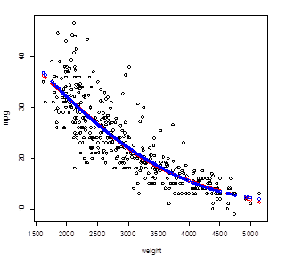
> plot( weight,mpg )

> Yhat_poly2 = fitted.values( poly2 )

> points( weight, Yhat_poly2, col="red", lwd=3 )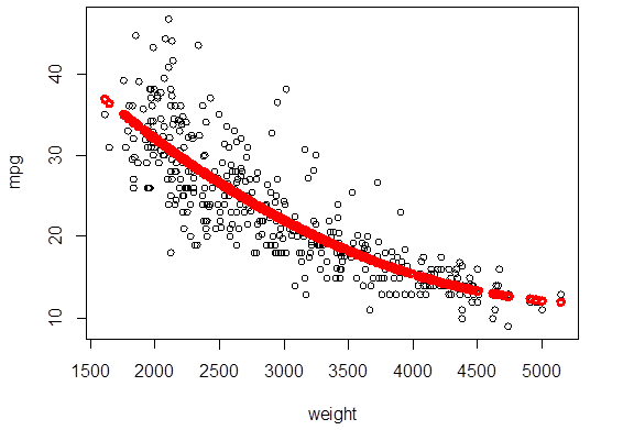

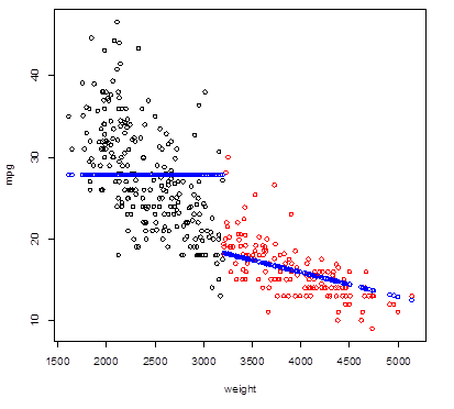
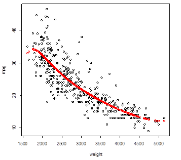
2. Broken Line – fitting different models on different intervals of X.

> n = length(mpg); # From the residual plot, the trend

> Group = 1*(weight > 3200) # changes around weight = 3200 lbs

> plot(weight, mpg, col = Group+1 ) # Red points correspond to heavier cars

> broken_line = lm( mpg ~ weight : Group ) # Interactions allow different slopes

> Yhat_broken = predict(broken_line) # Fitted values

> points( weight, Yhat_broken, lwd=2, col="blue" ) # Add fitted values to the plot

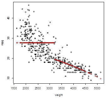
# Quadratic polynomial fit does not improve the picture

> broken_quadratic = lm( mpg ~ (weight + I(weight^2)) : Group )

> Yhat_broken_quadratic = predict(broken_quadratic)

> plot(weight,mpg); points( weight, Yhat_broken, lwd=2, col="brown" )

3. Splines – smooth connection at knots.

> install.packages("splines")

> library(splines)

> spline = lm( mpg ~ bs(weight, knots=3200) ) # In this lm, we defined the basis and knots

> Yhat_spline = predict(spline) # Fitted values

> plot(weight,mpg); points( weight, Yhat_spline, col="red" )

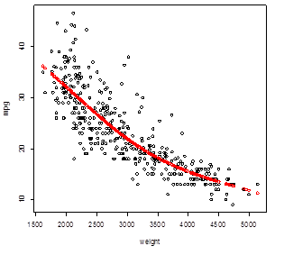
# This spline is almost the same as the quadratic polynomial regression!

> points( weight, Yhat_poly2, col="blue" )

# Add more knots?

> spline = lm( mpg ~ bs(weight, knots=c(2000,2500,3200,4500)) )

> Yhat_spline = predict(spline)

> plot(weight,mpg); points( weight, Yhat_spline, col="red" )

4. Cross-validation

> library(boot)

# Compare these four models by K-fold cross-validation, with K=n/4 groups, deleting 4 units at a time.

> reg = glm( mpg ~ weight )

> poly2 = glm( mpg ~ poly(weight,2) )

> spline1knot = glm( mpg ~ bs(weight, knots=3200) )

> spline4knots = glm( mpg ~ bs(weight, knots=c(2000,2500,3200,4500)) )

> cv.glm( Auto, reg, K=n/4 )$delta[1]

[1] 18.84014

> cv.glm( Auto, poly2, K=n/4 )$delta[1]

[1] 17.51702

> cv.glm( Auto, spline1knot, K=n/4 )$delta[1]

[1] 17.59429

> cv.glm( Auto, spline4knots, K=n/4 )$delta[1]

[1] 17.81641

# The quadratic polynomial model wins. Splitting X range into segments for the splints did not make much difference.

5. Smoothing Splines

5a. Fitting a smoothing spline

> attach(Auto); plot(weight,mpg); attach(splines);

> ss5 = smooth.spline(weight, mpg, df=5)

> lines(ss5, col="red", lwd=3)

> ss25 = smooth.spline(weight, mpg, df=25)

> lines(ss25, col="blue", lwd=3)

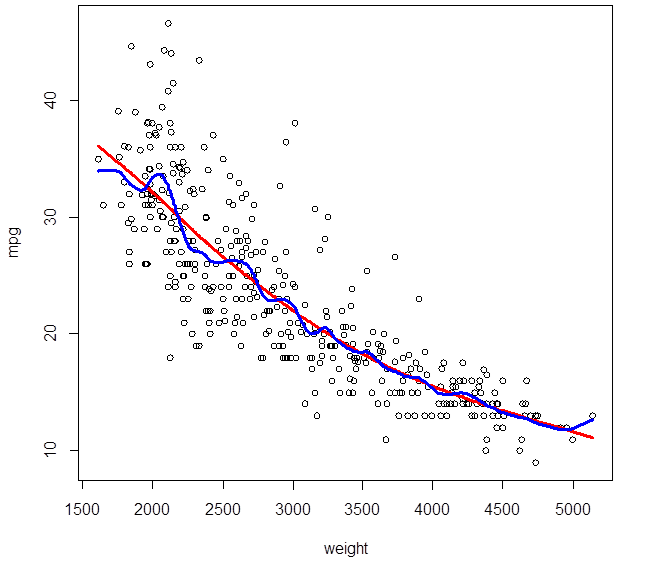
# A spline with (an equivalent of) 5 degrees of freedom is very smooth, its flexibility is limited by small df. A spline with 25 df is probably too flexible, too wiggly. The optimal df can be determined by cross-validation.

5b. Prediction error and cross-validation

> n = length(mpg); Z = sample(n,200); attach(Auto[Z,]); # This will be training data of size 200 (for example)

> ss5 = smooth.spline(weight, mpg, df=5) # Fit the spline using training data only

> attach(Auto);

> Yhat = predict(ss,x=weight)

> names(Yhat) # Notice: prediction consists of two parts – predictor x and

[1] "x" "y" # predicted response y. We can call them as Yhat$x and Yhat$y.

> mean(( Yhat$y[-Z] - mpg[-Z] )^2) # Then, compute prediction mean-squared error on test data

[1] 16.58982 # This is the cross-validation error for a spline with df=5

R also has a built-in cross-validation tool for smoothing splines. It uses the leave-one-out method (LOOCV, or jackknife)

> smooth.spline(weight, mpg, df=5, cv=TRUE)

Smoothing Parameter spar= 1.046238 lambda= 0.01789013 (11 iterations)

Equivalent Degrees of Freedom (Df): 5.000653

Penalized Criterion: 5974.815

PRESS: 17.59263 # This error (PREdiction Sum of Squares) is computed by LOOCV method

5c. Choosing the optimal degrees of freedom

We’ll fit smoothing splines of various df and choose the one with the smallest prediction error.

> cv.err = rep(0,50); Auto.train = Auto[Z,];

> for (p in 1:50){

+ attach(Auto.train); ss = smooth.spline(weight, mpg, df=p+0.01) # DF should be > 1

+ attach(Auto); Yhat = predict(ss, weight)

+ cv.err[p] = mean( (Yhat$y[-Z] - mpg[-Z])^2 ) }

> which.min(cv.err)

[1] 1

# This cross-validation chooses the smoothing spline with the equivalent of df=1.01

> ss = smooth.spline(weight, mpg, df=1.01)

> Yhat = predict(ss)

> plot(weight,mpg); lines(Yhat, lwd=3)